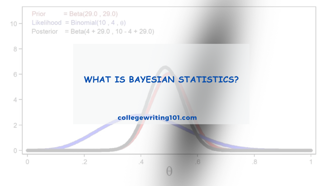
Bayesian statistics is an approach to data analysis built around a simple idea: as new evidence arrives, our beliefs should update accordingly. Unlike traditional (frequentist) methods, which treat parameters as fixed but unknown quantities, Bayesian statistics treats them as uncertain values described by probability distributions. This framework starts with a prior belief, combines it with observed data through a likelihood function, and produces an updated belief called a posterior distribution.
This way of thinking mirrors how people naturally reason. A doctor revises a diagnosis after new test results come in; an investor adjusts expectations after fresh market data appears. Bayesian statistics formalizes this process mathematically, offering a coherent way to quantify uncertainty rather than simply accepting or rejecting a hypothesis.
From medicine and machine learning to finance and scientific research, Bayesian methods have become central tools for decision-making under uncertainty, making them well worth understanding.
The Core Concept: Bayes’ Theorem
At the heart of Bayesian statistics lies a single equation that formalizes how to update beliefs in light of new evidence:
This deceptively simple formula connects four related quantities, each playing a distinct role in the reasoning process.
Breaking Down the Components
- Posterior probability, P(A∣B): The updated probability of event A occurring, given that event B has been observed. This is the answer we’re solving for—our revised belief after accounting for new evidence.
- Likelihood, P(B∣A): The probability of observing evidence B if A is true. This term measures how well the evidence fits the hypothesis.
- Prior probability, P(A): The initial probability of A before any new evidence is considered. This reflects existing knowledge, previous studies, or reasonable assumptions.
- Marginal probability, P(B): The overall probability of observing evidence B under all possible scenarios. It acts as a normalizing constant, ensuring the posterior probability is scaled correctly between 0 and 1. It is often expanded as:
A Worked Example: Medical Testing
Consider a disease that affects 1% of a population. A diagnostic test correctly identifies the disease 95% of the time (sensitivity) and correctly identifies healthy individuals 90% of the time (specificity). If a person tests positive, what is the probability they actually have the disease?
Let:
- = has the disease, so
- = tests positive
- (true positive rate)
- (false positive rate, since specificity is 90%)
First, calculate :
Now apply Bayes’ Theorem:
Despite a positive result, there is only about an 8.76% chance the person actually has the disease. This counterintuitive outcome illustrates why the prior probability matters so much: when a condition is rare, even a fairly accurate test produces more false positives than true positives in absolute terms.
Why This Matters
This example demonstrates the central strength of Bayesian reasoning: it forces explicit consideration of prior probabilities rather than relying solely on the accuracy of a single test or observation. Ignoring the prior—a mistake known as the base rate fallacy—can lead to serious misinterpretations in fields ranging from medical diagnostics to legal reasoning and machine learning classification.
Key Terms in Bayesian Statistics
| Term | Definition |
|---|---|
| Prior distribution | The probability distribution representing beliefs about a parameter before observing data. Can be informative (based on prior research) or non-informative (minimal assumptions). |
| Likelihood function | A function describing how probable the observed data is for different values of the parameter. Not itself a probability distribution over the parameter. |
| Posterior distribution | The updated probability distribution of the parameter after combining the prior with the observed data via the likelihood. |
| Marginal likelihood (evidence) | The total probability of the observed data, averaged over all possible parameter values. Serves as a normalizing constant in Bayes’ Theorem. |
| Posterior predictive distribution | The distribution of future observations, obtained by averaging predictions over the posterior distribution of the parameter. |
| Credible interval | A range within which a parameter falls with a specified posterior probability (e.g., a 95% credible interval). Distinct from a frequentist confidence interval in interpretation. |
| Conjugate prior | A prior distribution that, when combined with a particular likelihood, produces a posterior distribution of the same family (e.g., Beta-Binomial, Normal-Normal). |
| Non-informative prior | A prior chosen to have minimal influence on the posterior, often used when little prior knowledge exists. |
| Hyperparameter | A parameter of a prior distribution itself (e.g., the shape parameters of a Beta prior), as opposed to a parameter of the underlying model. |
| Bayes factor | A ratio comparing the likelihood of the data under two competing hypotheses or models, used for Bayesian hypothesis testing and model comparison. |
| Markov Chain Monte Carlo (MCMC) | A class of algorithms used to approximate posterior distributions when they cannot be calculated analytically. |
| Credible region | The multivariate generalization of a credible interval, used when more than one parameter is being estimated simultaneously. |
How Bayesian Statistics Works
With the core terminology established, it’s useful to walk through the practical process of Bayesian inference from start to finish. The following steps outline how a Bayesian analysis typically proceeds, illustrated with a running example.
Step 1: Define the Parameter of Interest
Identify the unknown quantity to be estimated. This might be a population mean, a proportion, a regression coefficient, or any other parameter governing the process under study.
Example: Suppose a researcher wants to estimate , the true proportion of customers who prefer a new product design over the old one.
Step 2: Specify a Prior Distribution
Choose a prior distribution, , that reflects existing knowledge or assumptions about the parameter before collecting new data. This may come from previous studies, expert judgment, or a deliberately uninformative choice if little is known.
Example: Based on similar past product launches, the researcher assumes a Beta(2, 2) prior, reflecting a mild expectation that preference is close to 50% but with considerable uncertainty.
Step 3: Collect Data and Define the Likelihood
Gather observed data and construct a likelihood function, , describing how probable that data is for different values of .
Example: A survey of 40 customers finds that 28 prefer the new design. Since each response is a binary outcome, the likelihood follows a Binomial distribution:
Step 4: Apply Bayes’ Theorem to Compute the Posterior
Combine the prior and likelihood to obtain the posterior distribution:
Example: Because the Beta distribution is conjugate to the Binomial likelihood, the posterior is also Beta-distributed. Starting with a Beta(2, 2) prior and observing 28 successes out of 40 trials:
Step 5: Summarize the Posterior Distribution
Once the posterior is obtained, summarize it using relevant statistics: the posterior mean, median, or mode, along with a credible interval to express uncertainty.
Example: The posterior mean is calculated as:
A 95% credible interval, computed from the Beta(30, 14) distribution, might span approximately 0.54 to 0.81, indicating strong but not absolute confidence that the new design is preferred by a majority of customers.
Step 6: Update the Model as New Data Arrives
One of the defining features of Bayesian analysis is that the posterior from one round of data can serve as the prior for the next. As additional observations become available, the process repeats, refining the estimate continuously rather than requiring a fresh analysis each time.
Example: If a second survey of 20 more customers is conducted, the current posterior, Beta(30, 14), becomes the new prior, and the cycle continues.
Step 7: Use the Posterior for Decision-Making or Prediction
The final posterior distribution can inform decisions directly, whether through point estimates, interval estimates, or posterior predictive distributions that forecast future observations.
Example: The researcher might conclude that there is strong evidence supporting a company-wide rollout of the new design, while still accounting for the residual uncertainty reflected in the credible interval.
Bayesian vs Frequentist Statistics
Statistics has long been shaped by two competing philosophies of inference: the Bayesian and frequentist approaches. While both aim to draw conclusions from data, they differ fundamentally in how they define probability and interpret results.
Philosophical Differences
The frequentist approach treats probability as the long-run frequency of an event across repeated trials. Parameters are considered fixed but unknown quantities, and inference relies on the behaviour of estimators across hypothetical repeated samples. The Bayesian approach, by contrast, treats probability as a degree of belief that can be assigned to parameters themselves, allowing prior knowledge to be formally incorporated and updated as new data arrives.
Key Points of Comparison
| Aspect | Frequentist Statistics | Bayesian Statistics |
|---|---|---|
| Definition of probability | Long-run frequency of an event | Degree of belief or confidence |
| Parameters | Fixed, unknown constants | Random variables with distributions |
| Use of prior information | Not incorporated | Explicitly incorporated via prior distribution |
| Main output | Point estimates, p-values, confidence intervals | Posterior distributions, credible intervals |
| Interpretation of intervals | Confidence interval reflects long-run capture rate over repeated sampling | Credible interval gives direct probability that parameter lies within range |
| Hypothesis testing | Null hypothesis significance testing (NHST), p-values | Bayes factors, posterior probabilities |
| Computation | Often simpler, closed-form solutions | Often requires simulation methods like MCMC |
| Sample size sensitivity | Requires larger samples for reliable inference | Can incorporate prior information to inform estimates with smaller samples |
| Subjectivity | Considered more objective, avoids explicit priors | Requires choosing a prior, which can be seen as subjective |
A Practical Illustration
Consider testing whether a new drug is more effective than a placebo. A frequentist analysis would calculate a p-value, testing whether the observed difference in outcomes is unlikely to occur by chance under a null hypothesis of no effect. A Bayesian analysis, instead, would compute a posterior probability that the drug is effective, directly incorporating any prior evidence from earlier trials and expressing the result as a probability statement about the treatment effect itself.
Which Approach Is Better?
Neither approach is universally superior, and the choice often depends on context, computational resources, and the nature of the question being asked. Frequentist methods remain dominant in many regulatory and industrial settings due to their long-established conventions and simplicity. Bayesian methods, meanwhile, have gained popularity in fields such as machine learning, genetics, and clinical trials, where incorporating prior knowledge and quantifying uncertainty directly offer clear practical advantages.
In practice, many statisticians now view the two frameworks as complementary tools rather than rival ideologies, each suited to particular problems and questions.
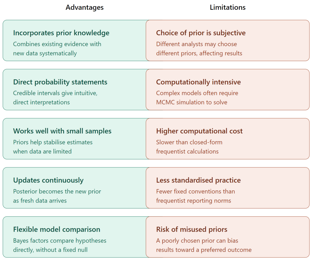
Advantages and Limitations of Bayesian Statistics
Real-World Applications of Bayesian Statistics
1. Healthcare & Clinical Trials
Bayesian methods are especially valuable in medicine, where decisions are high-stakes and data is often limited or noisy.
- Diagnostic Testing: Bayesian inference updates the probability of a disease given prior knowledge (e.g., prevalence) and observed symptoms or test results. This is the mathematical foundation of how clinicians reason about false positives and negatives.
- Clinical Trial Design: In January 2026, the FDA published draft guidance formally accepting Bayesian methodology as a legitimate approach for primary inference in clinical trials—particularly for rare diseases, pediatric populations, and fast-moving areas like oncology. This allows researchers to incorporate prior evidence and adapt trial designs based on interim results.
- Medical Genomics: Tools like Mutect2 and Strelka, used to identify genetic variants from DNA sequencing data, rely heavily on Bayesian frameworks underneath the hood to distinguish true mutations from sequencing errors.
- Medical Speech-to-Text: Purpose-built Bayesian optimization has helped clinical transcription models achieve a 3.44% word error rate in noisy hospital environments, significantly reducing documentation errors that can lead to misdiagnosis.
2. Quantitative Finance
Finance is a natural fit for Bayesian thinking because markets are noisy, data is limited, and decisions carry real monetary risk.
- Portfolio Allocation (Black-Litterman Model): Developed at Goldman Sachs in 1990, this model starts with market equilibrium as a “prior” and blends it with an investor’s subjective views (with confidence levels) to produce more stable, diversified portfolios than classical mean-variance optimization. It remains a standard tool in asset management.
- Strategy Evaluation: Bayesian inference computes full posterior distributions for metrics like Sharpe ratio or maximum drawdown, giving investors honest credible intervals rather than misleading point estimates. A strategy with a backtest Sharpe of 1.5 might actually have a 95% credible interval of (0.4, 2.6).
- Regime Detection: Bayesian Hidden Markov Models detect shifts between market regimes (e.g., high vs. low volatility, risk-on vs. risk-off), outputting the probability of being in each regime at any given time to guide risk management.
- Credit Risk: Bayesian networks are considered viable tools for credit risk prediction in terms of both performance and interpretability, though production implementations at major institutions often blend them with other ML approaches.
3. Marketing & A/B Testing
Bayesian A/B testing is increasingly preferred over traditional frequentist methods because it allows continuous monitoring, incorporates prior campaign knowledge, and produces directly interpretable probabilities (e.g., “Variant B has an 89% probability of being better than A”). This is especially useful with small sample sizes or when quick decisions are needed.
4. Machine Learning & AI Infrastructure
- Hyperparameter Optimization: Bayesian optimization (using Gaussian processes) is the industry standard for tuning expensive models—such as large neural networks—by intelligently exploring the search space rather than brute-force grid search.
- Recommendation Systems: Netflix and other platforms use Bayesian probabilistic models to handle data sparsity and cold-start problems, combining prior knowledge about user behavior with observed interactions.
- Gaussian Processes: These provide flexible, probabilistic regression and classification with built-in uncertainty estimates, widely used in robotics, sensor fusion, and scientific modeling where knowing how uncertain a prediction is matters as much as the prediction itself.
5. Natural Language Processing
Bayesian neural networks and topic models (like Latent Dirichlet Allocation) are used for sentiment analysis, machine translation, and topic modeling. They improve performance by incorporating prior linguistic knowledge and continuously updating as new text data arrives.
6. Weather & Climate Science
Bayesian deep learning combines computer vision imagery with historical weather patterns to improve forecasting. The probabilistic framework naturally handles the chaotic, uncertainty-rich nature of atmospheric systems.
7. Industrial Process Control & Root Cause Analysis
Object-oriented Bayesian networks are deployed in complex continuous processes (e.g., pulp and paper manufacturing) to perform real-time diagnostics, risk assessment, and decision support under uncertainty. These systems recommend corrective actions and explain their reasoning, learning from operator feedback over time.
8. Autonomous Systems & Robotics
While still largely in the research phase, Bayesian frameworks provide the theoretical backbone for uncertainty-aware perception and decision-making in autonomous vehicles and robots navigating unpredictable environments.
Common Bayesian Methods and Models
1. Bayesian Parameter Estimation
Conjugate Priors
When the prior and posterior belong to the same distribution family, inference becomes analytically tractable.
| Likelihood | Conjugate Prior | Posterior | Use Case |
|---|---|---|---|
| Bernoulli/Binomial | Beta(α, β) | Beta(α + successes, β + failures) | A/B testing, conversion rates |
| Normal (known σ²) | Normal(μ₀, τ₀²) | Normal(μₙ, τₙ²) | Sensor calibration, measurement errors |
| Poisson | Gamma(α, β) | Gamma(α + Σxᵢ, β + n) | Call center arrivals, web traffic |
| Multinomial | Dirichlet(α) | Dirichlet(α + counts) | Topic modeling, market share |
Why it matters: In production A/B testing at companies like Netflix, a Beta(1,1) uniform prior updates to Beta(1+conversions, 1+non-conversions), giving a full posterior distribution over conversion rates without any sampling.
Markov Chain Monte Carlo (MCMC)
When conjugacy doesn’t hold, MCMC approximates the posterior by drawing correlated samples.
- Metropolis-Hastings: Proposes new parameter values and accepts/rejects based on the posterior ratio. Works for any model but mixes slowly in high dimensions.
- Gibbs Sampling: Samples each parameter conditional on all others. Efficient when conditional distributions are tractable (e.g., Bayesian linear regression, hierarchical models).
- Hamiltonian Monte Carlo (HMC): Uses gradient information to propose states, dramatically improving exploration in high-dimensional spaces. The workhorse of Stan and PyMC.
Deployment note: HMC in Stan/PyMC is now GPU-accelerated (NumPyro achieves 11× speedups), making it viable for production ML pipelines.
Variational Inference (VI)
Approximates the true posterior p(θ|x) with a simpler variational distribution q(θ) by minimizing KL divergence.
- Mean-Field VI: Assumes parameters are independent (q(θ) = ∏ qᵢ(θᵢ)). Fast but misses correlations.
- Full-Rank VI: Captures parameter covariances. More accurate, slightly slower.
- Automatic Differentiation VI (ADVI): Stan’s default—transforms to unconstrained space and optimizes.
Trade-off: VI is 10–100× faster than MCMC but yields approximate posteriors. Preferred for large-scale applications (e.g., recommendation systems at Netflix).
2. Bayesian Regression & Classification
Bayesian Linear Regression
Extends ordinary least squares with priors on coefficients:
y=Xβ+ϵ, ϵ∼N(0,σ²)
β∼N(μ₀,Σ₀), σ²∼Inv-Gamma(α,β)
Advantage over frequentist: Produces credible intervals for predictions, not just point estimates. In finance, this yields honest uncertainty bounds for portfolio returns.
Bayesian Logistic Regression
Same framework with a sigmoid link:
P(y=1∣X)=1+e−Xβ1
With a Laplace prior (L1 equivalent), it performs automatic feature selection—useful when p >> n (many features, few samples).
Bayesian Neural Networks (BNNs)
Place priors over network weights:
w∼N(0,σw²I), y∼N(fw(x),σy²)
Key methods:
- MCMC Dropout: Uses dropout at test time as approximate Bayesian inference. Lightweight, widely used.
- Bayes by Backprop: Variational inference over weights. More principled but computationally heavier.
- Laplace Approximation: Fits a Gaussian around the MAP estimate. Fast post-hoc uncertainty.
Use case: Medical imaging, autonomous driving—anywhere model confidence must be calibrated.
3. Probabilistic Graphical Models
Bayesian Networks (Directed Acyclic Graphs)
Represent joint distributions as products of local conditional probabilities:
P(X1,…,Xn)=∏i=1nP(Xi∣Pa(Xi))
Applications:
- Medical diagnosis: Infer disease probability from symptoms and test results.
- Credit risk: Model dependencies between financial indicators.
- Root cause analysis: In pulp/paper manufacturing, object-oriented Bayesian networks diagnose process faults in real time.
Markov Random Fields (Undirected)
Useful when relationships are symmetric (e.g., image segmentation, spatial data).
Hidden Markov Models (HMMs)
Latent state sequences with Markov dynamics:
zt∼P(zt∣zt−1), xt∼P(xt∣zt)
Bayesian HMMs place priors on transition and emission probabilities. In finance, they detect market regimes with full uncertainty quantification.
4. Hierarchical (Multilevel) Models
Pool information across groups while allowing group-specific variation:
yij∼N(αj+βjxij,σ2)
αj∼N(μα,σα²), βj∼N(μβ,σβ²)
Partial pooling: Groups with little data “borrow strength” from the global distribution; groups with lots of data dominate their own estimates.
Use cases:
- Clinical trials: Pooling across hospital sites or patient subgroups.
- Education: Student performance across schools.
- Marketing: Ad effectiveness across regions.
5. Gaussian Processes (GPs)
Define distributions over Functions rather than parameters:
f(x)∼GP(m(x), k(x, x′))
Common kernels:
- RBF/Squared Exponential: Smooth, infinitely differentiable.
- Matérn: Less smooth, more realistic for physical processes.
- Periodic: For cyclical patterns.
Key property: Predictions come with full uncertainty:
f∗∣X,y,x∗∼N(μ∗,σ∗2)
Applications:
- Bayesian optimization: GPs model the expensive objective function.
- Robotics: Trajectory planning with uncertainty-aware collision avoidance.
- Sensor fusion: Combining noisy measurements with known physics.
6. Bayesian Optimization
Optimizes expensive black-box Functions by building a probabilistic surrogate (usually a GP) and using an acquisition function to balance exploration vs. exploitation.
Acquisition Functions:
Table
| Function | Behavior | When to Use |
|---|---|---|
| Expected Improvement (EI) | Maximize E[max(f(x) – f⁺, 0)] | General-purpose, robust |
| Probability of Improvement (PI) | P(f(x) > f⁺ + ξ) | When you need guaranteed improvement |
| Upper Confidence Bound (UCB) | μ(x) + κσ(x) | When exploration is cheap |
| Entropy Search | Reduce uncertainty about the optimum | Very expensive evaluations |
Industry standard: Used by Google, Amazon, and OpenAI for hyperparameter tuning of deep learning models.
7. Bayesian Nonparametrics
Dirichlet Processes (DP)
Allow the number of mixture components to grow with data:
G∼DP(α,G0)
Use case: Clustering where the number of clusters is unknown (e.g., customer segmentation, topic discovery).
Gaussian Process Latent Variable Models (GPLVM)
Nonlinear dimensionality reduction with uncertainty.
8. State-Space & Sequential Models
Bayesian Filtering (Kalman Family)
For dynamic systems with hidden states:
- Kalman Filter: Linear-Gaussian systems. Optimal, closed-form.
- Extended Kalman Filter (EKF): Local linearization for mildly nonlinear systems.
- Unscented Kalman Filter (UKF): Sigma-point propagation, better for strong nonlinearities.
- Particle Filters: Sequential Monte Carlo for arbitrary distributions. The “gold standard” when nothing else works.
Applications: GPS navigation, robotics localization, econometric forecasting.
9. Bayesian Topic Models
Latent Dirichlet Allocation (LDA)
Generative model for documents:
θd∼Dirichlet(α), ϕk∼Dirichlet(β)
zd,n∼Multinomial(θd), wd,n∼Multinomial(ϕzd,n)
Extensions:
- Dynamic Topic Models: Topics evolve over time.
- Hierarchical LDA: Topics form a tree structure.
Deployment: News recommendation, patent analysis, scientific literature mining.
10. Modern Variants & Hybrids (2024–20
| Method | Innovation | Use Case |
|---|---|---|
| Neural Processes | Combine GPs with neural networks for meta-learning | Few-shot prediction |
| Bayesian Deep Learning with Normalizing Flows | Flexible posterior approximations | High-dimensional uncertainty |
| Closed-Form UQ | Analytical uncertainty without sampling | Real-time systems |
| Bayesian Transformer Layers | Uncertainty in attention mechanisms | NLP with calibrated confidence |
Choosing the Right Me
| Situation | Recommended Approach |
|---|---|
| Small data, need exact posteriors | Conjugate priors |
| Medium data, complex model | HMC (Stan/PyMC) |
| Big data, need speed | ADVI / SVI |
| Expensive function evaluations | Bayesian Optimization + GP |
| Time-series with hidden states | Bayesian Filtering / HMM |
| Many related groups | Hierarchical models |
| Unknown number of clusters | Dirichlet Processes |
| Need interpretable causal structure | Bayesian Networks |
| Deep learning + uncertainty | BNNs (MCMC Dropout / Bayes by Backprop) |
The unifying principle across all these methods is the same: encode what you know before seeing data (the prior), update with evidence (the likelihood), and reason about what remains uncertain (the posterior).
Example of Bayesian Thinking in Everyday Life
1. The Morning Commute: “Should I Leave Now?”
Prior belief: Based on years of experience, you believe there’s a 20% chance traffic is bad this morning.
New evidence: Your navigation app shows a 5-minute delay on your usual route.
Likelihood: If traffic is actually bad, you’d expect to see a delay 80% of the time. If traffic is normal, you might still see a minor delay 10% of the time.
Posterior update: Using Bayes’ theorem, your belief shifts from 20% to roughly 64% that traffic is bad. You decide to leave 10 minutes early.
This is exactly what a Bayesian Kalman filter does in your GPS—continuously updating position estimates with noisy sensor data.
2. The Spam Folder: “Is This Email Junk?”
Prior: 90% of emails to your address are spam (your inbox baseline).
Evidence: The subject line contains “URGENT: Account Suspended” and a suspicious link.
Likelihood: Phishing emails use this exact phrasing about 30% of the time; legitimate emails use it perhaps 0.1% of the time.
Posterior: The probability this is spam jumps to 99.7%. Your email provider’s Bayesian spam filter (like the classic Paul Graham implementation) made this calculation automatically.
The filter started with generic priors and continuously updated them based on which emails you marked as spam—classic Bayesian learning.
3. The Restaurant Review: “Will I Like This Place?”
Prior: A new Thai restaurant opens. You know nothing, so you assign it a neutral prior—say, 50% chance you’ll enjoy it, based on your general liking of Thai food.
Evidence 1: First review is glowing. Your belief shifts to 70%. Evidence 2: Second review mentions “too salty.” Your belief drops to 55%. Evidence 3: A trusted friend whose taste matches yours raves about it. Your belief jumps to 85%.
Key insight: Not all evidence is equal. Your friend’s opinion carries more weight (higher likelihood ratio) than a random stranger’s—just as Bayesian hierarchical models weight data sources by their reliability.
This is also how Netflix’s recommendation engine works: it combines your viewing history (prior) with what similar users watched (evidence), weighting each source by its predictive power.
4. The Medical Test: “Do I Actually Have This?”
This is the classic textbook example because it so powerfully demonstrates base rate neglect.
Prior (base rate): The disease affects 1 in 1,000 people in your demographic. P(Disease) = 0.1%.
Test result: You test positive. The test is 99% accurate.
Intuitive (wrong) reaction: “I’m basically 99% likely to have it.”
Bayesian calculation:
- P(Positive | Disease) = 99% (true positive rate)
- P(Positive | No Disease) = 1% (false positive rate)
- Out of 1,000 people: 1 truly has it and tests positive; ~10 healthy people also test positive.
Posterior: P(Disease | Positive) = 1 / 11 ≈ 9%.
You are far more likely to be a healthy false positive than a true case. This is why doctors don’t test everyone for rare diseases indiscriminately—the prior matters enormously.
The same logic applies to genetic variant calling in medical genomics: tools like Mutect2 use Bayesian frameworks to distinguish real mutations from sequencing noise by incorporating base rates of different mutation types.
5. The Job Interview: “How Did I Do?”
Prior: Based on your preparation and the company’s selectivity, you estimate a 30% chance of getting an offer before the interview.
Evidence: The interviewer smiled, asked about your start date, and mentioned “the team.”
Likelihood: If they plan to offer you the job, these signals occur 70% of the time. If they don’t, they occur 15% of the time.
Posterior: Your probability of an offer rises to roughly 67%.
Then: You hear nothing for two weeks. You update again—silence is more likely if they’re not interested. Your posterior drifts back down.
This sequential updating is exactly what Bayesian filtering does: each new piece of evidence revises your belief, and the previous posterior becomes your new prior.
6. The Weather Forecast: “Should I Bring an Umbrella?”
Prior: Historical data says it rains 20% of the time in July.
Evidence: The morning forecast says 60% chance of rain.
Likelihood: When it actually rains, the forecast predicts rain 80% of the time. When it doesn’t rain, the forecast still predicts rain 30% of the time (forecasters hedge).
Posterior: Given a rain forecast, the actual chance of rain is about 40%—not 60%. You might skip the umbrella if you’re only going out briefly.
This is why probabilistic weather models use Bayesian deep learning to combine satellite imagery with historical patterns, outputting calibrated uncertainty rather than single-point predictions.
7. The “Gut Feeling”: Why Experts Seem Intuitive
A veteran doctor glances at a patient and thinks “something’s wrong.” A seasoned mechanic hears an engine and knows the problem. A poker player folds despite a decent hand.
These aren’t mystical instincts—they’re compressed Bayesian inference. Years of experience built strong priors. New evidence (a subtle symptom, an engine pitch, an opponent’s tell) gets evaluated against those priors instantly. The expert’s posterior updates so fast it feels like intuition.
The difference between a novice and an expert is largely the quality of their priors. A beginner chess player evaluates a position from scratch; a grandmaster’s prior, built from 10,000 games, makes the evaluation nearly instantaneous.
Tools and Software for Bayesian Analysis
1. Probabilistic Programming Languages (PPLs)
These are the core engines that let you define Bayesian models in code and run inference automatically.
Stan
The gold standard for Bayesian inference. Stan compiles models written in its own modeling language into highly efficient C++ code, then runs Hamiltonian Monte Carlo (HMC) with the No-U-Turn Sampler (NUTS) or variational inference (ADVI). It is the engine behind many higher-level packages.
- Best for: Complex hierarchical models, reliable MCMC, production-grade inference
- Interfaces: R (RStan), Python (CmdStanPy), Julia, MATLAB, and more
- Key feature: Automatic step-size and mass-matrix adaptation for robust sampling
PyMC
A modern, comprehensive probabilistic programming framework for Python. PyMC lets you write models in friendly Python syntax and compiles them through PyTensor for CPU, GPU, or JAX backends. It includes NUTS, ADVI, ABC, SMC, and Gaussian processes out of the box.
- Best for: Python-native Bayesian modeling, from beginners to advanced users
- Key integrations: ArviZ for visualization, Bambi for high-level mixed models
- Key feature:
pm.do()andpm.observe()for causal inference and counterfactuals
NumPyro
A lightweight probabilistic programming library built on JAX. NumPyro implements NUTS and stochastic variational inference (SVI) with automatic differentiation, enabling GPU/TPU acceleration and just-in-time compilation.
- Best for: Research-grade modeling where JAX speed and differentiability matter
- Key feature: Composable inference with JAX transforms, excellent for large-scale or deep Bayesian models
Turing.jl
A Julia-native probabilistic programming language with syntax close to mathematical notation. Turing supports discrete parameters, stochastic control flow, and is fully interoperable with the Julia scientific computing ecosystem.
- Best for: Julia users who want flexibility and performance in one package
- Key feature: Native support for models with discrete latent variables (unlike Stan)
TensorFlow Probability
A library for probabilistic reasoning and statistical analysis built on TensorFlow. It provides layers, distributions, bijectors, and MCMC/variational inference tools that integrate directly into TensorFlow and Keras pipelines.
- Best for: Production ML systems already using TensorFlow; scalable Bayesian deep learning
- Key feature:
TransformedDistributionand bijectors for exact change-of-variables density modeling
2. High-Level Interfaces & Wrappers
These packages sit on top of PPLs to make common modeling tasks easier.
brms
An R package that provides a familiar lme4-style formula interface for fitting Bayesian generalized multilevel models. It translates your R formula into Stan code automatically, then runs Stan sampling behind the scenes.
- Best for: R users who want Bayesian regression without writing Stan code
- Supported models: Linear, robust linear, count, survival, ordinal, zero-inflated, hurdle, mixture, and distributional regression
- Key feature: One-line model specification with full Stan posterior diagnostics
Bambi
A Python package similar to brms, providing a high-level formula interface for Bayesian regression built on PyMC. It handles mixed-effects models, splines, and distributional regression with minimal code.
- Best for: Python users who want R-style formula syntax for Bayesian models
3. Specialized Inference Engines
JAGS
“Just Another Gibbs Sampler” — a cross-platform engine for the BUGS modeling language. JAGS uses Gibbs sampling and is particularly strong for hierarchical models where conjugacy can be exploited.
- Best for: Users familiar with BUGS syntax; models with discrete latent variables
- Latest version: JAGS 4.3.2 (March 2023)
- Key feature: Extensible — users can write custom Functions, distributions, and samplers
BUGS
The original Bayesian inference Using Gibbs Sampling software, developed at the MRC Biostatistics Unit in Cambridge. OpenBUGS and WinBUGS are the main variants. Historically foundational, though many users have migrated to JAGS or Stan.
- Best for: Legacy models, teaching, and specific applications where BUGS dialect is standard
INLA
Integrated Nested Laplace Approximation — an R package for fast, approximate Bayesian inference for Latent Gaussian Models. Instead of MCMC, INLA uses deterministic approximations, making it orders of magnitude faster for the model classes it supports.
- Best for: Spatial and spatiotemporal models, large latent Gaussian problems where MCMC is too slow
- Key feature: Direct access to posterior marginals without sampling; strong spatial support via
inlabru
4. GUI-Based & Teaching Tools
JASP
A free, open-source statistical software with a point-and-click interface that offers both frequentist and Bayesian analyses. Developed at the University of Amsterdam, it produces publication-ready APA-formatted output.
- Best for: Students, researchers new to Bayesian methods, and anyone who prefers a GUI
- Key feature: Dynamic updating of all results; drag-and-drop interface; integrated with the Open Science Framework
jamovi
A free, spreadsheet-style statistical application built on R. While not exclusively Bayesian, it provides accessible statistical analysis with a clean GUI and can connect users gradually to the broader R ecosystem.
5. Visualization & Diagnostics
ArviZ
The standard Python library for exploratory analysis of Bayesian models. It works with PyMC, Stan, NumPyro, and others, providing trace plots, posterior distributions, forest plots, and convergence diagnostics (R-hat, ESS).
bayesplot
An R package for plotting Bayesian models, tightly integrated with Stan and brms. It provides a rich library of diagnostic and posterior visualization Functions.
FAQs
Is ChatGPT Bayesian?
No. ChatGPT is mainly based on deep learning (neural networks), not purely Bayesian statistics. However, it uses probabilities, which are conceptually related to Bayesian ideas.
When should I use Bayesian statistics?
Use it when:
You have prior knowledge or beliefs
Data is limited
You need to update predictions as new data comes in
Is AI based on Bayesian statistics?
Partly. Some AI models use Bayesian methods, but most modern AI (like deep learning) relies more on neural networks than Bayesian approaches.